In Part 1 I described the k-means clustering algorithm and some of its uses along with a quick Python implementation. Going forward I recommend using the scikit-learn implementation.
Now let's see k-means in action!
Image Segmentation
One use of clustering is to segment images:
For example, in computer graphics, color quantization is the task of reducing the color palette of an image to a fixed number of colors k. From: k-means clustering (Wikipedia)
Given an image, we can use k-means clustering to find similar colours in the image, and re-draw it with fewer colours. This has uses in data compression for example.
This is the example I'll run through today.
We'll take this image of a puppy:
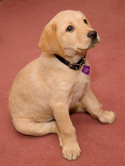
Puppy image from Greg on Flickr and redraw it in much fewer colours using k-means clustering.
The Data
Let's start by defining our data. To represent this problem, we take each pixel in the image as a data point whose 3 features are the R, G and B values of the pixel.
For this particular image this gives us a dataset with 3 columns and 43,680 rows. Some of the pixels are the same colour, but we've still got over 10,000 unique colours in our image.
Running K-means
It is conceivable that we can group similar colours together and redraw the same image with fewer colours in a way that we can still tell what is in the image. This would reduce the amount of information needed to represent the image (and therefore the filesize) without visibly losing much detail.
Once we have our dataset (the details of extracting the pixel values will be in the accompanying Jupyter notebook) running the algorithm with scikit-learn is easy:
from sklearn.cluster import KMeans

kmeans = KMeans(n_clusters=k)
# our dataframe (df) is the image data
clusters = kmeans.fit_predict(df)
# "clusters" is a vector with a cluster assignment for each data point (pixel)
df['cluster'] = clusters
# use the K cluster centroids as new colours to represent the image
colours = [tuple([int(c) for c in x]) for x in kmeans.cluster_centers_]
In this instance the cluster centroids are points in 3D space, where the 3 dimensions are R, G and B, so the centroids can be thought of as colours themselves.
That means once we have the cluster assignment for each pixel, plus the centroid as the associated colour value, we can reconstruct our image pixel by pixel to get the $k$-colour representation.
The same image with only 3 colours looks like this:
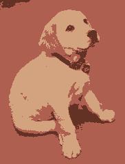
The same puppy drawn with only 3 colours
As you can clearly see, we've reduced the number of colours required, and incidentally also reduced the filesize threefold, without losing too much information. The image is still clearly a puppy, despite the fact that we've only used 3 colours.
When we use 16 colours the image starts to resemble the original in much more detail:
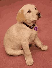
A 16-colour puppy
You can still see the background isn't smooth but we're getting close. In fact, we would get to an image that is indistinguishable from the original by using far less than the original 10,000 colours.
Here is the Jupyter notebook for drawing puppies.
I have a couple of points left to raise, namely some practical tips when using clustering.
Choosing K
How would we know which point to stop at? When is $k$ at its optimal value?
As I mentioned in part 1, this is usually somewhat subjective, but there are some general heuristics.
In this case we could do it by visual inspection. That is, we could say $k$ is high enough when we are no longer visually able to tell the difference between the original and the redrawn images.
Not all datasets will lend themselves to visual inspection like this though.
We can use what's called the elbow method to evaluate when to stop.
For each value of $k$ you want to evaluate how much of the variance in your data is explained by the configurations of those $k$ clusters. This value increases for each value of $k$, but the idea is that we stop increasing $k$ when increasing it gives us diminishing returns.
Let's think of the two extremes. When $k$ = 1, it means every point will belong to the same cluster. This configuration explains 0% of the variance in your data, because it says all your data points are the same. Then $k$ is equal to the number of data points you have, it means every point will belong to its own cluster. This configuration explains 100% of the variation in your data because it says each of your data points is different from every other one. A value in between will explain some % of the variation, because it will say some data points are equal to some other data points, and different from some others.
Here's a good explanation of the elbow method, although it uses the "error" for each $k$ value, so the graph is upside down compared to the "variance explained" metric I discussed above.
Either way, there is usually an "elbow" where the increase/decrease is suddenly less sharp. That's usually a good point to stop and use that value for $k$.
Normalisation
As I mentioned in the Self-Organising Maps tutorial, in practice you will want to normalise your data so all features are on the same scale. This is also true of k-means clustering. If all features are on the same scale, each feature will "contribute" to the algorithm equally, otherwise a feature with much larger values will dominate the others.
In the case of colours, the R, G, and B values are all on the same scale (0 to 255) so this is not necessary, but in real world examples your features will often be on different scales.
See more information on this in Sebastian Raschka's machine learning FAQ.
K-means and clustering in general have many more uses, and I hope these puppies have piqued your interest!

About David
I'm a freelance data scientist consultant and educator with an MSc. in Data Science and a background in software and web development. My previous roles have been a range of data science, software development, team management and software architecting jobs.
